Climate Models & Predictions for the Future

"Time drops in decay,
Like a candle burnt out,
And the mountains and woods
Have their day, have their day".
-W. B. Yeats, "The Moods"

Suggested Readings:

• World Meteorological Organization Intergovernmental Panel on Climate Change, "Climate Change: The IPCC Scientific Assessment", Cambridge, 1990.
• White, J. C., "Global Climate Change Linkages: Acid Rain, Air Quality, and Stratospheric Ozone", Elsevier, 1989.
• Ahrens, C. Donald, "Meteorology Today", 6th ed., Brooks/Cole Publishing Co., 1999.

We wish to learn:

• What can we say about potential future climate change?
• How do climate models work and what are their predictions for the future?

1. The Paleoclimate Record

Ice Core Measurements

Scientists have developed a technique by which global mean sea-surface temperatures can be deduced from measurements of the isotopic fractionation of oxygen in ice cores. This technique provides us with estimates of sea-level air temperatures over the past 160,000 years.

In order to establish the reliability of such measurements, paleoclimatologists have conducted a number of tests to calibrate this "paleoclimate thermometer" in the ice.

Figure 1 shows an intercalibration of two sets of ice core isotopic measurements, one from Byrd Station in the Southern Hemisphere, and the other from Camp Century in the Northern Hemisphere. A decrease of one part per million (ppm) in the d¹⁸ O measurement is equivalent to a reduction in temperature of approximately 1.5^oC at the time that the water evaporated from the oceans.

Clearly the two sets of measurements are correlated, both showing the temperature reduction of the most recent Pleistocene glacial outbreak between 60,000 and 15,000 years ago. The warming trend to the present interglacial period started around 15,000 years ago. The dates for such measurements are obtained using models of ice deposition and flow.

Measurements of other isotopic ratios (such as light hydrogen to heavy hydrogen) in ice also provide important climate information.

The ice-core oxygen isotope measurements are complemented by studies of the composition of ancient air trapped in bubbles in the ice. The top panel of Figure 2 is a micro-photograph of an ice-core slice, clearly showing trapped bubbles. The ice is brought back to a laboratory and heated carefully in a vacuum chamber (to avoid contamination by modern air), releasing the ancient air for analysis.

The bottom panel of Figure 2 shows the results of ice bubble analysis for the atmospheric gas methane (CH4). The dots in the lower panel of Figure 2 represent ice measurements of methane, while the asterix represents atmospheric measurements of the methane abundance global average from the late 1970's. These analyses have shown that methane concentrations have hardly changed over most of the 160,000 year period, staying at values near 750 parts per billion. At about the time of the industrial revolution, however, methane concentrations rose, due in part to the production of the gas by enteric processes in cattle, anaerobic processes in rice paddies, and other human-driven activities. The recent rise in methane from pre-industrial levels is more than a factor of 2!

We have seen how ice cores can provide information on both temperatures and atmospheric composition for ancient times. Let's put the two pieces of evidence together and assemble a more detailed 160,000 year record of climate. Figure 3 shows the time series of ice-core data for temperature (oxygen isotope measurements) and for carbon dioxide and methane abundances (ice bubble measurements). The most recent rise in methane and carbon dioxide is not shown on this scale. The comparison is dramatic - all three curves show similar features!

The top panel of Figure 3 shows the temperature data for the past 180,000 years. The present (near left-hand side of graph) is relatively warm compared with the last period when glaciers covered Michigan ~18,000 years ago. The period of extensive cooling was marked by repeated advances and retreats of the glaciers.

Both methane and carbon dioxide correlate with temperature - i.e., an increase in temperature is associated with an increase in the abundance of both these two gases. It is unclear whether the gas abundance changes are a consequence of the temperature changes or vice versa.

Correlations such as these are difficult to interpret. It is hard to unravel the chain of cause and effect when a poorly understood feedback process is at play. Additional evidence for these processes are sought.. As we shall soon discuss, useful additional evidence comes from a study of changes in the Earth's orbit.

Figure 2. Ancient air found in bubbles trapped in ice cores (above, temporary picture) may be carefully analyzed to provide information on the atmospheric composition.

Figure 3. Correlations between the Ice Core measurements of paleoclimate temperatures and abundances of methane and carbon dioxide.

Deep Sea Sediment Analysis

The paleoclimate record discussed above goes back about 160,000 years. Compared with the history of the Earth, this is a very short period of time indeed. We can go back farther, however, using measurements made of oxygen isotope ration in deep sea cores, drilled from the ocean floor.

Analysis of oxygen isotopic ratios of ocean and atmospheric water oxygen isotopes has shown ocean surface sea water becomes enriched in heavy oxygen due to the temperature-dependent evaporation process. It follows that sea creatures living in these waters will possess shells containing more heavy oxygen. The proportion of heavy oxygen in sea shells (consisting of calcium carbonate -- CaCO₃) will go up in years when the temperature is colder and will go down in years when the temperature is warmer (exactly the opposite behavior to the heavy oxygen in glacial ice discussed above). This isotopic fractionation process was demonstrated in the laboratory by Harold Urey (the same Urey who was Stanley Miller's thesis advisor). In the 1950's, Urey performed a controlled laboratory experiment with plankton. He grew these tiny shelled creatures at different temperatures and was able to demonstrate the temperature dependence of the oxygen isotopic fractionation in the shells (i.e. the higher the temperature of the water, the smaller the ratio of heavy-to-light oxygen in the calcium carbonate of the shells).

Several deep sea cores have since been analyzed to determine the oxygen isotopic ratio of ancient calcium carbonate. It is from these these measurements and careful calibrations that we can obtain a record of sea surface temperatures that goes back almost 1 million years!

Figure 5 shows the million-year paleoclimate record, together with more detailed records of successively later times. To generate this figure, additional information has been used from the techniques noted on the right hand side of the diagram. It should be remembered that 1 million years represent only about one fiftieth of one percent of the Earth's lifetime.

We start our discussion with the one-million-year time series (Figure 5, Panel e). Note that the record from the deep sea sediments shows cycles of alternating cold and warm periods with a period of about 100,000 years. Superimposed on this long-term cycle are multiple excursions on shorter time scales. Clearly Michigan has been subject to many periods of glaciation over the past million years!

If we focus on the last 150,000 years only (Panel d), we see the glacial/interglacial features already indicated in Figure 3. The recent warming trend started in ~15,000 years ago (Panel c), when the glaciers last left Michigan. This warming coincides with the development of human civilization.

Panel c also shows a phenomenon of interest to us - the Younger Dryas. This was a short-lived period lasting about 700 years that occurred 10,000 years ago, when the general warming trend was interrupted by a sudden cooling. The term Younger Dryas was coined from the herbaceous plant "dryas" that covered much of the landscape during the colder time period. Evidence for this sudden cooling came from the study of ancient pollen grains found in sediments, which showed a abrupt change from pre and postglacial forests to glacial shrubs and then back again. This climate "jump" was also seen in ice core measurements of CO₂. The Younger Dryas provides dramatic evidence for rapid jumps in climate. We shall see in a later lecture, this phenomenon should be taken as a warning of possible things to come if rapid human-induced climate change continues.

Panel b of Figure 5 shows the record of the past 1,000 years. The climate about 1,000 years ago was relatively warm and dry (wine was grown in England!). We know from history that this was also the period that the Vikings ran out of room in Scandinavia and colonized Greenland (remember, it doesn't look very green now). Unfortunately for them, the period of relatively clement climate was replaced by colder conditions during the famous "Little Ice Age" and Greenland became uninhabitable again. The Little Ice Age is celebrated in paintings by Breugel of frozen rivers and streams in Holland. We are clearly seeing a connection between human activities and climate.

The most recent 200 years are shown in Panels a and b. During this time, global human activity signifigantly expanded and industrial revolution flourished. The graphs show that warming has continously increased (with a few interruptions), resulting that the 1980's has been the warmest decade of this of the century.

2. Causes of Paleoclimate Change

It is clear from the above discussion that climate change is constant - and that it occurs at all time scales. We next need to discuss the causes for paleoclimate change. In this discussion, we will start with the most ancient changes and move to the more recent changes. Of course, much of what follows is speculation and our picture will undoubtedly change as new paleo-climatological techniques are developed.

Although the basic causes of climate change are still not fully understood, many clues have been collected. Possible causes include:

• Changes in solar output
• Changes in Earth's orbit
• Changes in the distribution of continents
• Changes in the concentration of Greenhouse Gases in the atmosphere

We will separately consider climate changes over several different time scales: 1) the long term (100's million years); 2) medium term (1 million years); 3) short term (160,000 years) and 4) modern period (last few centuries).

Long-Term Changes

The long term (100's million years) paleoclimate record, shown in Figure 6, is characterized by relatively few, isolated glacial outbreaks - the great Ice Ages. We need to seek a factor, or a combination of factors, that could change the climate in this way over these long periods. The time scales and nature of the record argue against solar output and Earth's orbit changes to explain the great Ice Ages.

Radiation from the Sun is not constant, but varies at least by ~0.1 to 0.2%. There is a 22 year cycle of sunspots that causes a similar 22 year cycle of solar radiation. This cycle is thought by many scientists to play a minor role in climate change (though this is still subject to heated debate). Over longer periods, it is known that solar activity changes (as recorded by number of sunspots). It is interesting to note, for example, that during the "Maunder Minimum" (~1645-1715) few if any sunspots were seen. This corresponds to the peak time of the Little Ice Age.

Sunspot cycles have much too short a period to explain the great Ice Ages and we need to look for variations in solar output over much longer time intervals. Here we can appeal to plasma physics and to what is known about stellar evolution. Solar physicists believe that stars like the Sun brighten slowly over billions of years. In fact, the sun is thought to have been 30% dimmer 3 billion years ago than it is today. This slow increase in solar radiation with time does not help us explain the great Ice Ages, however, since one would then expect a record that followed the slow curve of solar radiation rather than the episodic plot of Figure 6. Although it is based on fundamental physical principles, the dim early sun is not an immediately helpful concept for paleoclimatologists. It is often called the "Faint Young Sun Paradox" since, if the sun were really that dim, one would have expected quite a different story for planetary evolution.

Changes in the nature of the Earth's orbit around the Sun, known as Milankovitch Cycles, occur over too short time scales to explain the long term climate change. These cycles are discussed below with reference to the medium-term changes.

So what then caused the Great Ice Ages? Let us consider the possibility of changes in the atmospheric greenhouse effect.

Our best guess today is associated with the very slow process known as "Plate Tectonics" and its influence on the atmospheric greenhouse effect. We will discuss Plate Tectonics in greater detail later on in this course. For the moment, it is sufficient to know that the continents (plates) "drift" on top of a fluid substrate over geologic time. When plates collide, some material can be pushed under the Earth's crust in a process known as "subduction", leading to increased volcanism.

Over the time scale of 300 million years (back to the last known Great Ice Age - the Gondwanan, see Figure 6), the continental plates have moved greatly. Figure 7a shows the distribution of continents today, together with the areas showing evidence of Gondwanan glaciation.

Figure 7b shows the locations of the continents ~300 million years ago when they were assembled into the great supercontinent Pangaea. It can be seen that the regions showing glaciation were all assembled near the South Pole.

The question remains as to why the temperatures dropped. Perhaps the answer lies in changes in the natural (non-biogenic) production rate of carbon dioxide - the number one greenhouse gas. We know that CO₂ is produced in volcanoes and in the mid-ocean trenches. It is lost by being slowly absorbed in the oceans. Both of these processes are very slow - about the right time scales to explain the great Ice Ages.

A drop in the production rate of carbon dioxide by volcanism would reduce the atmospheric greenhouse effect and lead to lower temperatures. We may speculate that the Gondawanan Ice Age started when the moving continental plates first assembled in Pangea (like bumper cars), they had to go through a readjustment period before drifting apart again. Perhaps, during the readjustment period, the production of carbon dioxide dropped, leading to the Gondwanan Ice Age.

Figure 8 shows how carbon dioxide is produced by volcanism and sea-floor spreading. During times of rapid spreading, increased volcanic activity, coupled with higher ocean levels and reduced chemical weathering of rocks, may promote global warming by enriching the CO₂ content of the atmosphere. Similarly, global cooling may result from stalled or slowed spreading.

Medium-Term Changes

The medium term changes in paleoclimate temperatures were illustrated by Figure 5e, above. This period, called the Pleistocene, was characterized by semi-regular advances and retreats of the glaciers during the most recent (and continuing) Great Ice Age.

The best clue for explaining these changes comes from a consideration of the Milankovitch cycles, changes in the orbital characteristics of the Earth.

Milankovitch Cycles

There are three types of orbital change of relevance to our discussion. These were first described by the Yugoslavian astronomer Milutin Milankovitch who first proposed the idea of a climate connection in the 1930's.

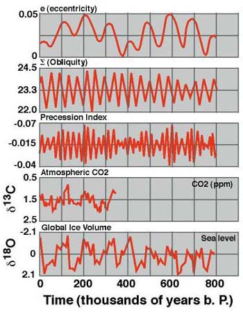
The basic premise of the theory is that, as the Earth travels through space, three separate cyclic movements combine to produce variations in the amount of solar energy falling on the Earth. Figure 9 illustrates the first type of orbital change, dealing with the changes in the shape of the Earth's orbit (eccentricity) as the Earth rotates about the Sun. The more eccentric the orbit the more elliptical the orbital shape.

It turns out that the Earth's orbit goes from quite elliptical to nearly circular in a cycle with a period of ~100,000 years. Presently, we are in a period of low eccentricity (~3%) and this gives us a seasonal change in solar energy of ~7%. When the eccentricity is at its peak (~9%), the "seasonality" reaches ~20%. In addition a more eccentric orbit will change the length of seasons in each hemisphere by changing the length of time between the vernal and automnal equinoxes.

The second Milankovitch cycle takes about 41,000 years to complete and involves changes in tilt (obliquity) of the Earth's axis (Figure 10). Presently the Earth's tilt is 23.5°, but the 41,000 year cycle varies from ~22° to 24.5°. The smaller the tilt, the less seasonal variation there is between summer and winter at middle and high latitudes.

For small tilt, the winters would tend to be milder and the summers cooler. This would lead to more glaciation.

The third cycle is due to precession of the spin axis (as in a spinning top) and occurs over a ~23,000 year cycle. Presently, the Earth is closest to the Sun in January and farther away in July. Due to precession, the reverse will be true in ~11,000 years. This will give the Northern Hemisphere more severe winters.

Figure 11 shows the correlation of the Milankovitch cycles with the paleoclimate records for the past million years. There is a good correlation, between periods of low eccentricity and glacial periods. A detailed view of the interglacial periods of the past ~160,000 years also shows evidence of the 41,000 year and 23,000 years cycles.

Other factors which work in conjunction with the Earth's orbital changes include:

• The amount of dust in the atmosphere
• The reflectivity of the ice sheets
• The concentration of greenhouse gases
• The changing characteristics of clouds
• The rebounding of land, having been depressed by ice.

The Milankovitch cycles may help explain the advance and retreat of ice over periods of 10,000 to 100,000 years. They do not explain what caused the Ice Age in the first place.

When all the Milankovitch cycles (alone) are taken into account, the present trend should be towards a cooler climate in the Northern Hemisphere, with extensive glaciation.

Short-Term Changes

The glacial-interglacial variations observed over the 160,000 year record of Figure 6 are explained in part by solar forcing due to the Milankovitch theory. However, it remains to explain the observed correlation between the greenhouse gases methane and carbon dioxide, shown in Figure 3.

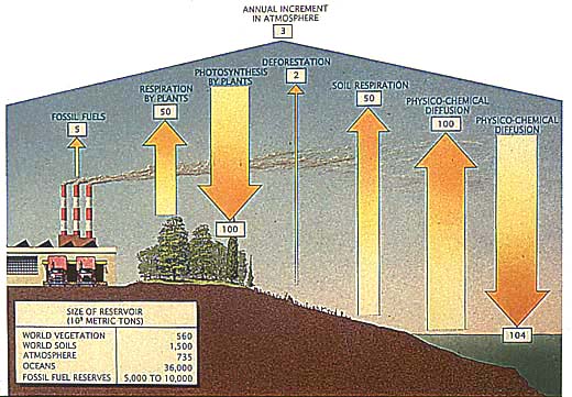
The correlation between methane, CO₂ and temperature could perhaps be explained by invoking a temperature dependence to the cycling of CO₂ and methane through the environment. Figure 12 shows examples of fluxes and reservoirs for CO₂. The main reservoir is the ocean. A dependence of the flux from the ocean to temperature (the higher the temperature, the greater the flux to the atmosphere) could explain the correlation for CO₂, while a similar temperature dependence for decomposition could explain the methane correlation.

Modern Changes

Modern changes in temperature and carbon dioxide are shown in Figures 13 and 14. Modern methane variations have been shown in Figure 2.

It is clear from these figures that rapid changes are underway - at rates far exceeding anything discussed so far.

It must be assumed that human activities (known as Anthropogenic Effects) are dominating the present changes.

The past century has seen an increase in the global mean temperature of 0.8^oC.

Some of the variations seen are a consequence of volcanic eruptions. Such events can emit large quantities of dust into the stratosphere where sunlight can be intercepted for a period of a few years.

The upward trend may also be a consequence of the increasing levels of carbon dioxide, methane and CFCs put into the atmosphere through various anthropogenic processes.

Figure 15 shows multi-year measurements of carbon dioxide abundances from a single location in Hawaii. The strong yearly signal (peak in winter months, minimum in summer months) can be seen, together with the strong increase due to anthropogenic effects. The causes and consequences of this rise will be the subject of much additional discussion in this course. Figure 16 shows the modern climate records for methane and carbon dioxide. Both species show a strong yearly cycle (peaking in the winter months). The cycle is more pronounced in the Northern Hemisphere due to the preponderance of human activities and continents there.

3. Climate Models

A number of sophisticated global climate models have been developed over the past 15 years for the purpose of predicting future climatic change. The most highly developed models are three-dimensional and time dependent and divide the globe up into a series of interacting boxes. The reservoirs and fluxes of importance are coded into the computer program which then solves the conservation equations of mass, momentum, and energy in order to calculate the evolving state of the atmosphere/hydrosphere system.

In general, models such as these must be validated against observations. This is done sometimes by running the model backwards in time to specify past, known climates. However useful, these predictive models have to constantly checked against experimental data to insure accurate results.

Climate models are often used to predict the climate of an Earth in which the carbon dioxide concentration has doubled. This is a prospect very likely to occur within the next 50-100 years, given the current increasing rates of anthropogenic CO₂.

Below are some results of climate models run under twice the current global carbon dioxide concentration.The model predictions for future climate are based on forward estimates of the rate of fossil fuel consumption. They also include prescriptions for the multiple interactions among clouds, land, oceans, etc.:

• Climate model predict a climate that is significantly hotter and more humid than now. (Figure 17).
• Climate models predict an increase in the mean sea level of 6 meters over the next 100 years. Different scenarios give different results, but the basic trend is the same (Figure 18).
• Climate Models also predict increases of 4 degrees over the same 100 year interval. It must be noted that the exact prediction is dependent on the assumptions used for fossil fuel consumption rate (see Figure 19).

4. Summary 

1.       A paleoclimate record has been developed using different techniques, stretching back over 2 billion years. The Earth was warmer than at present for most of this time, punctuated by infrequent Ice Ages.

2.       The Great Ice Ages may have been caused by processes associated with continental drift and greenhouse warming.

3.       The interglacial periods are related to orbital changes described by the Milankovitch cycles, among other factors.

4.       In recent times, temperature changes and greenhouse gas abundances are correlated. Rapid global warming is underway and models have been developed to predict the effects of these changes.

 Copyright ©Regents of the University of Michigan