Natural Selection and Mutation - The Case of the Peppered Moth
 Learning Objectives
One of the most critical questions that we face today is how will the species on Earth adapt, or can they adapt, to the rapid global changes brought on by anthropogenic forces. This question is important for society because many species are critical for human survival and food security, are already endangered and on the brink of extinction, or are at the core of cultural values and the sense of community (e.g., think of the central role that bowhead whales play for many communities of Indigenous People in the Arctic). Species adapt to new environmental conditions by changing their behavior (within limits), by mutation, or by altering the expression of their genes. This adaptation can be relatively rapid for some species, but certainly not all species, and in today's lab we will examine the biology behind a famous case of relatively rapid adaptation of the peppered moth to environmental pollution.
The purpose of this lab exercise is to model the effects of natural selection on the appearance and genetic make-up of a natural population (the peppered moth). We will construct a STELLA model for this population that incorporates the basic principles of population genetics, as described in lecture and here in the lab exercise. Please note that for simplicity, the STELLA model you will work with today assumes that black and white are the only moth color phenotypes possible (we will ignore the gray moth phenotype Dr. Badgley mentioned in lecture for now).
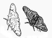
Figure 1
The peppered moth (Biston betularia)
Before we begin, we will need to define some important genetic terminology:
- Alternative forms of a gene are called alleles; All sexually reproducing organisms have two alleles - one inherited from each parent
- The genetic constitution of an individual is called its genotype
- The physical expression of a genotype is called the phenotype
- If two alleles are identical, an individual is said to be homozygous for that gene; if two alleles are different, the individual is said to be heterozygous
- A dominant allele has
such a strong phenotypic effect in heterozygous individuals that it
conceals the presence of the weaker (recessive) allele
Introduction
The case of the peppered
moth (Biston betularia) is a classic example of
evolution through directional selection (selection favoring extreme
phenotypes). Prior to the industrial revolution in
The allele (version of the gene) for dark body color is dominant, which means that a moth possessing at least one such allele will have a dark body. To have a light body, the moth has to have both alleles for light body color.
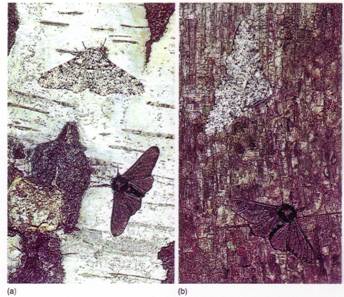
Figure 2
Dark and light phenotypes of the peppered moth on dark bark (right) and lichen covered (left) trees
Dark moths were at a distinct disadvantage, however, due to their increased vulnerability to bird predation. Thus the frequency of the dark allele was very low (about .001%), maintained primarily by spontaneous mutations from light to dark alleles. By 1819, the proportion of dark moths in the population had increased significantly. Researchers found that the light-colored lichens covering the trees were being killed by sulfur dioxide emissions from the new coal burning mills and factories built during the industrial revolution. Without the light background of the trees, the light moths were more visible to vision-oriented predators (birds). They were losing their selective advantage to the dark moths, which, against the trees’ dark bark background, were less visible to birds. In 1848, the dark moths comprised 1% of the population and by 1959 they represented ~90% of the population. So, in 100 years the frequency of dark moths increased by 1000 fold!
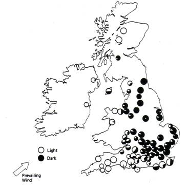
Figure 3
Composition of various populations
of the peppered moth in the
In this exercise, we
will construct a model simulating the effects of differential predation
pressures on a hypothetical peppered moth population. To do this, we will need
to incorporate the genetics of moth body color into a population dynamics
model. We are assuming that body color is the only trait that confers any
significant selective advantages on peppered moths.
Building the Model
As you build this model, you will have to use ghosts ![]() to create copies for duplicate variables. However, it is extremely important to make the "Total Moths" converter in the lower part of the model the original. Then, all the other ones can be ghosts copied off of it. Make sure the ghost versions of the stocks are in the lower part of the model with the original "Total Moths" converter.
to create copies for duplicate variables. However, it is extremely important to make the "Total Moths" converter in the lower part of the model the original. Then, all the other ones can be ghosts copied off of it. Make sure the ghost versions of the stocks are in the lower part of the model with the original "Total Moths" converter.
To use the Ghost icon, click on the icon then click on the variable you want to copy and add it to the model. The ghost converter should look shadowy, with a dotted outline. You should only edit the original variables in the model, not the ghosts.
Note: Always connect all necessary components to a "converter" or "flow" before entering equations
Ultimately, the structure of your model will look like this:
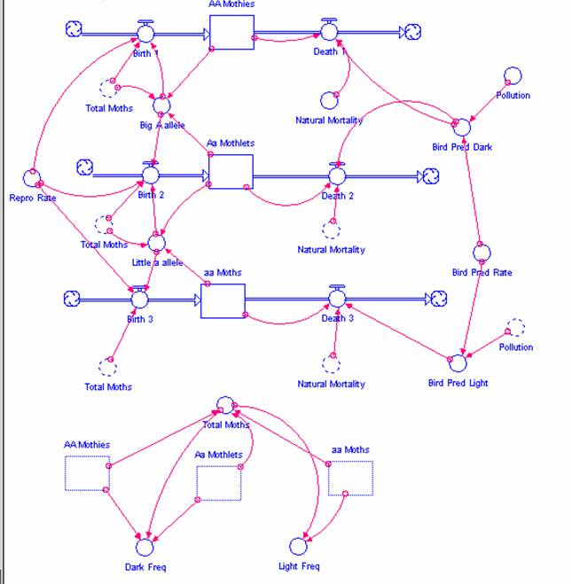
Figure 4
STELLA model of the peppered moth
As with any system, we must first identify and define the stocks and flows of the system.
Stocks
Start to build your model by creating the following three stocks. We have three different genotypes represented in our model:
- AA mothies: homozygous dominant moths that are dark in color
- Aa mothlets: heterozygous moths that are also dark in color
- aa moths: homozygous recessive moths that are light in color
Note: STELLA will not let you repeat variable names. Because STELLA is not case sensitive, it doesn’t distinguish between the names "aa moths" and "Aa moths," so make sure to vary them (i.e. "moths" vs. "mothlets.")
Flows
The flows of our genotypic subpopulations are birth and death. First, take a look at the birth flows: Components on the right side of the equation are given below, and these will be your converters. First create the flows, then create the converters necessary for entering the equations into the flows, and then connect these converters to the flows with connectors. Finally, input the correct equations. At this point, you will not have entered any values for your converters, that will happen below.
- birth1 = (repro rate * total moths) * (big A allele^2)
- birth2 = (repro rate * total moths) * (2*big A allele*little a allele)
- birth3 = (repro rate * total moths) * (little a allele^2)
In these flows, the birth rate is calculated by multiplying the reproduction rate of the total population with the frequency of occurrence specific to that genotype.
The allele frequencies are calculated as:
- big A allele = ( (2*AA mothies/total moths) + (Aa mothlets/total moths) ) / 2
- little a allele = ( (2*aa moths/total moths) + (Aa mothlets/total moths) ) / 2
The term for total
moths is calculated by using the ghost ![]() to make
copies of the 3 stocks and adding them together:
to make
copies of the 3 stocks and adding them together:
- total moths = AA mothies + Aa mothlets + aa moths
Also define variables that calculate the relative frequencies of dark moths (AA and Aa) and light moths (aa):
- dark freq = (AA mothies + Aa mothlets) / total moths
- light freq = aa moths / total moths
Now look at the death flows for the stocks:
- death1 = AA mothies * (natural mortality + bird predation dark)
- death2 = Aa mothlets * (natural mortality + bird predation dark)
- death3 = aa moths * (natural mortality + bird predation light)
The death flows incorporate a natural mortality rate as well as death resulting from predation by birds. Notice that the bird predation rates are different for dark and light moths. These two different predation rates are defined by:
- bird predation light = pollution * bird pred rate
- bird predation dark = bird pred rate - ( pollution * bird pred rate )
Bird predation rate and pollution are both proportions between 0 and 1. Notice that with high rates of pollution, bird predation light is higher, while bird predation dark is highest when pollution is low.
Below are the constants and rates that we have chosen for this model:
- repro rate = .055
- natural mortality = .045
- bird pred rate = .04
- pollution = 0.0 (for now)
- AA mothies = 250
- Aa mothlets = 500
- aa moths = 250
Set up two graphs for viewing results. The first (graph 1) should display dark freq and light freq (this is the phenotype graph). Set up the second graph (graph 2) to display numbers of AA mothies, Aa mothlets, and aa moths (this is the genotype graph). The run specs for these runs are starting at 0.0 to 200.0 with a DT = 1.0, and the time units set for years. Next, set up numeric displays (icon that looks like a figure 8) to observe the numeric changes in allele frequencies (little a allele and big A allele.) Click the wrench icon then set the graph to multi-scale by clicking the multi-scale check box.
Investigating the System
Since pollution is the true driver of the change in genotype frequency in the peppered moth population, it is the variable that we are most interested in modifying. Pollution is a proportional term, i.e. if it is zero there is no pollution and when it equals 1, pollution is at a maximum.
Simulate the following three scenarios with your model. For each scenario, save graphs 1 and 2 and copy and paste them into your word document. Make sure to label each graph with the value of the pollution variable (or write it in a caption under the graph).
- First, run the model with no pollution (pollution = 0)[graphs #1&2].
- Next, run the model with maximum pollution (pollution = 1)[graphs #3&4].
- Finally, run the model with a changing pollution rate, which we can define graphically (as opposed to mathematically). Click on and open the pollution converter, and then select and click on the TIME function in the Built-ins list. (First delete the value in the equation box.) Now click on the graphical function tab, and then the Graphical Function checkbox at the top of the panel. Notice that the X axis is TIME and the Y axis is pollution.
Change the number at the top of the Y-axis to 1.0 to restrict the range of pollution to between 0 and 1. Make sure the X-axis ranges from 0 to 200, representing a time span of 200 years. Next, using your mouse (or typing in the desired output), draw an s-shaped graph that starts off at 0 (no pollution) and increases rapidly, then levels off at 1 (maximum pollution) halfway across the graph (i.e. TIME ~100).
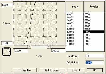
Figure 5
Screen Shot
Run the model under this pollution scenario, copy and paste the graphs that reflect a rise in pollution near year 100 [graphs #5&6].
Now vary the timing of the rise in pollution by shifting the position of the rise on the X-axis. Make two new graphs and note how the timing affects the dynamics of the different genotypes[graphs #7&8].
Questions
Question 1
- Turn in the graphs showing phenotypic (graph 1) and genotypic (graph 2) responses in the moth population for each of the scenarios that you've tested. [You should have eight graphs total at this point. Be sure to label your graphs].
- In a paragraph, describe the dynamics you observe in each scenario. Also, what happens to the genotypes and phenotypes of the moths when pollution suddenly increases in the system (talk about scenario 3)? Why?
Question 2
- Name and describe the effects of two significant assumptions we have made in the construction of this model.
- What would be the effect of relaxing (changing) these assumptions on the structure of the model AND the results of the model?
Question 3
- What would you expect to happen (in terms of genotypic and phenotypic frequencies) if pollution levels fluctuated widely?
- Check out your hypothesis by varying the pollution function (add some spikes and dips to make it highly variable), - Include your graphs [graphs #9&10, be sure they are labelled].
Question 4
- Considering the more complicated case of peppered moth color morphs described in lecture, what aspects of the model would you change if the genotype "Aa" made the moths gray (i.e. in between dark and light)?
- Adapt the structure of your model to reflect this change and include a screen shot. Note: We are not asking for you to enter equations or actually run the model - we only want you to change the structure of the model.
Question 5
- If you changed the pollution levels in your new model with dark, light, and gray moths, how would the new gray phenotype would fare? (Make a prediction)
- In your model, "life adapts to pollution levels and survives." Do you think this is representative of most real world situations? Explain.
As usual submit your one Word document as an attachment on Canvas, it should contain:
- Answers to questions 1-5, with associated graphs (you should have 10 total graphs for the entire assignment). PLEASE make sure to label all your graphs!
- Screenshot of your final model structure (Use screenshot from Question 4 which includes the gray moths)
- Copy and paste final equations of your final model (at bottom of your Word document)
Sources
Futuyma, Douglas J. 1979. Evolutionary Biology. Sinauer Associates,
Hartl, Daniel L. 1988. A Primer of Population Genetics, second edition. Sinuaer
Associates,