*Remember to save your work along the way in your Google Drive or U-M Dropbox. If you do not know how to do this ask your GSI.
*Stella is available on the computers in the fishbowl and in the Dana building.
Objective
Perhaps the most critical interaction of humans with our planet in the last 50 years is climate warming. Human activities have increased the temperature of our planet to the point where climate extremes have at times a severe and negative impact on human wellbeing. At the moment, society is looking to scientists to help understand why the planet is warming, how warm will the planet become, and what can we do to mitigate or adapt to this climate change. The goal of this class is to gain a working knowledge of, and an insight into, the processes of climate change and an understanding of what controls the temperature of our planet.
The natural systems (e.g., ecosystems, the climate system) that we need to understand are extraordinarily complex. Therefore, in order to study the response of these systems to change, it is necessary to reduce this complexity. We do this by creating models, which are simplified representations of reality. Modeling is the process of distilling complex systems down to their essential (and hopefully manageable) components, and then to examine these components in an integrated way - this is referred to as "systems thinking". In this lab, we first introduce some of the modeling concepts and tools (STELLA) that we will use throughout the course to study the response of dynamic systems to change, and we build a simple model of the input and output of water to a bathtub - this is called a "mass balance" model, which is a concept that is important for many aspects of this course. In this lab, we will apply that mass balance concept to an understanding of the energy balance of our planet in terms of the energy inputs and outputs that control Earth's temperature.
The Modeling Process
Modeling should be approached in a logical and ordered manner. Though following guidelines may seem tedious and unnecessary at times, it greatly increases the chances that your model will (a) work and (b) be a relatively accurate representation of the actual behavior of a real-life system.
At its essence, modeling is a 5-part process:
1. Define the Problem and the Goals of the Model
This is where most people get into trouble. Aside from programming problems, most models give incorrect results because (a) the system under study was not understood well enough or (b) the modeler did not have a clear idea of what the model was actually supposed to show. Make note of any assumptions needed to simplify the model at this stage.
2. Understand the Real Life System
Figure out the crucial components of the system. (These are represented as stocks, flows, converters and connectors in STELLA.) Exclude any components that are unnecessary. Keep the model as simple as possible, because unnecessary complexity will make the model difficult to understand or modify later on.
3. Build the Model
Sketch out the connections between model variables. Once you have made all of the relevant connections, use STELLA icons to build the model.
4. Test and Revise the Model
Run the model with different data in order to find out if it works, what its limitations are, and where and when it breaks down.
5. Verify the Model
Though not always possible, try to test your model against real world data.
Although we will not be strictly following every step of the above guideline in the development of the models in this lab, it is important that you keep them in mind as you develop models now and especially as you create and modify models in various labs this semester.
CREATE YOUR FIRST MODEL -- THE BATHTUB
The instructions listed below will guide you through the construction of your first computer model. You may want to refer to the Guide to Basic STELLA Features for help.
To illustrate basic modeling principles and introduce you to STELLA, we will construct a simple model of a typical bathtub. The goal of our modeling is to determine what flow is necessary to fill, but not overfill, our bathtub. Before we proceed with programming our model in STELLA, let’s think about the bathtub system. What is it that we want to describe? What physical laws govern our system? What inputs and outputs are there to our bathtub? What simplifications will we make to our model to make it tractable?
What is it that we want to describe? Because our goal is to fill the bathtub, we want to describe the water volume in the tub. This is our “state variable” that describes the condition of our system, and will have units of m^3.
Most bathtubs have a faucet and a drain. We must include these in our model. Flow from the faucet is the input; flow in to the drain is the output. The flow in will be equal to the rate of flow (m/s) times the area (m^2) of the faucet head. The flow out will be equal to the rate of flow (m/s) times the area (m^2) of the drain. Both of these are volume fluxes, and have units of m^3/s.
What physical laws govern our system? The volume of water in the bathtub is dependent upon the amount that comes in and the amount that flows out. We have just described a conservation law. It is this rule that will govern our model. (Strictly speaking, we should be conserving “mass” rather than “volume”. However, because the density of water in to and out of our bathtub is constant, we can make this simplification.) This idea of mass balance will be investigated later in the course.
What simplifications will we make to our model to make it tractable? One simplification is that we will ignore the temperature of the water in our tub. The density of water, that is the number of water molecules per m^3, is temperature dependent. Warm water has a lower density and, as a result, a larger volume than cold water. It turns out that this effect is pretty small and won’t have much consequence on our estimates. What other simplifications are we making?
Now that we have described the rules for our bathtub we can begin constructing it! Follow along with your GSI.
- Start Stella. A "New Model" blank page greets you. You can now start building your model.
- Construct a stock for the state variable. In the upper panel, click on the STOCK tool,
. Click again to place the stock on the page. Label your stock by typing in a name (e.g. Bathtub). Click on the stock icon, and a dialog box will appear on the right-hand side of the screen. Under this dialog box, click on the chi-squared symbol, 𝛘², to switch to the "Model View". Inside the Bathtub icon is an exclamation mark reminding you that an initial value is needed. In the "Equation" texbox, type 0 as the initial value. You can also add comments between curly brackets ({}) in the Equation field. It is very important to get into the habit of adding units! These should be added as comments. So type {m^3}, which represent cubic meters.
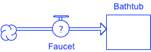
- Construct a flow that regulates water in to the bathtub. In the upper panel, click on the FLOW tool,
 . Move the pointer to the left of the Bathtub stock and click. You may need to drag the arrow into Bathtub so that the box darkens, indicating that the flow has been connected to the stock. Label your flow by typing in a name (e.g. Faucet). Your model should now look like this:
Make sure the flow is connected to the stock. If your model, looks like this:
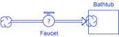
then the flow was not properly placed within the Bathtub stock.
The question mark in the Faucet flow tool above indicates that an input value is required. Click on Faucet, and enter an initial value of 0.01, the rate of water flow (m^3/s) from the faucet. Add units!
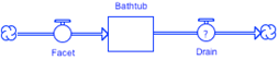
- Build a flow that regulates water out of the bathtub. Again, click on the FLOW tool. This time click to the right of the Bathtub stock. You many need to drag the arrow to the left to connect to the Bathtub stock. Label your flow by typing in a name (e.g. Drain). Your model should now look like this:
- Make an action connector that links the Bathtub and Drain icons. Unlike flow from the faucet, which is completely independent of the bathtub volume, flow down the drain depends on the volume of water in the bathtub. For example, if the bathtub is empty, there is no water to flow down the drain. To make this connection, click on the ACTION CONNECTOR tool,
 . Click in the Bathtub icon, and drag the arrow to the Drain icon, like this:
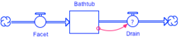
- The final step in the construction of our model is to define drain outflow (m^3/s). Click on the Drain icon. In the dialog box, click on Bathtub, then the multiplication sign (*), and finally type 0.01. Note that we have just defined the outflow as 1% of the bathtub volume. Add units!
- SAVE YOUR MODEL. Your career as a professional in any number of careers will be a lot happier if you remember to save your work often.
- Specify the run time for your model. You must tell STELLA how long to run your model. What is a reasonable length to fill a bathtub? We’ll choose 600 seconds. Under the MODEL pull-down menu, select Run Specs. In the dialog box, under Run Specs, set: "Start Time" = 0, "Stop Time" = 600, "DT" = 1 (de-select "Fractional"), "Sim Duration" = 1.5 seconds, and "Time Units" = seconds (This is not a default choice, you must type in "seconds"). Click OK.
- Set up a graph to view the model output. Click on the GRAPH icon,
 , and then on your workspace area. A dialog box will display showing the available variables that can be plotted. In the "Series List", click on the green "+" to add a new series. From the pop-up menu, select Bathtub to add it as the new series. Click OK to close the dialog box. Resize and move the window to a good location.
- MAKE A PREDICTION: how do you expect the water volume in the bathtub to change?
- Run the model. Under the MODEL pull-down menu, select "Run". The graph that appears should look like this:
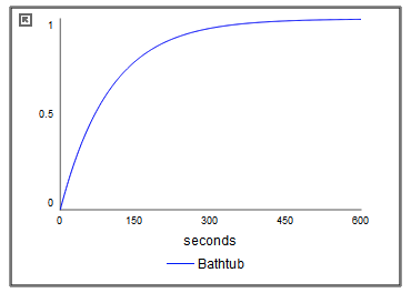
- Check your model results! What does the graph tell you? How full does the bathtub get? How long does it take? Do your model results make sense? Increase the flow from the faucet by 10 times. How does this change your results?
The STELLA modeling system is a user-friendly interface that allows you to build mathematical equations without getting bogged down in the details of programming and complex math. Take a look at the real workings of the model in the "Equation Viewer" (MODEL pull-down menu --> "Equation Viewer"). In this equations layer, the icons you created are translated into difference and differential formulas. Although you will not be expected to interpret the math in these equations, you should be able to see what relationships are being represented.
Summary of what we have learned thus far:
So far in this lab exercise we have learned what a model is, and how to construct a simple model in STELLA. In future exercises our models will be more complex, but will follow the general rules learned here.
EARTH ENERGY BALANCE MODEL
Objective
The sun radiates energy outward toward the planets, which provides light and
heat to the Earth. At the same time, the Earth radiates energy back into space.
In this exercise, we will use STELLA to create a model showing these energy
flows and the equilibrium that is reached. This model is relatively simple, yet
very powerful. It describes the temperature of our planet, one of the key factors
that has led to the evolution of life.
Figure 1
The sun
Part 1. Define the Problem and Goals of the Model.
The primary goals of this exercise are to illustrate the physical processes
that dictate the Earth’s temperature, and to create a model that accurately
predicts the radiative equilibrium temperature that maintained the early
Earth’s energy balance. It is important that you understand the basic
assumptions and conclusions of the model to understand how this process works
as a system, so that you can incorporate information learned later on and build
on your modeling skills.
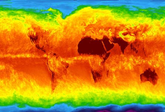
Figure 2
Picture of the infrared (IR) radiation being output from Earth
Part 2. Understand the Real Life System.
DO NOT START YOUR MODEL UNTIL YOU GET TO THE STEP BY STEP INSTRUCTIONS IN PART 3.
Read through the entire Part 2 before you start building the model.
Let’s first consider the stocks and flows that will comprise the heart of our model. The thing that accumulates in our system is energy. So we will represent Earth energy as a stock in our model. The processes affecting this stock are (1) Earth’s capture of solar radiation; and (2) the emission of infrared energy from Earth to space. We will represent these processes by flows into (solar to Earth) and out of (Earth to space) the Earth energy stock (Figure 3).

Figure 3
Initial components of the Earth energy balance model
Figure 4
Solar to Earth
Next, identify the radiation laws (see lecture notes) and other physical properties that govern these flows. We know that the amount of solar radiation reaching the Earth (or any other planet) is a function of its diameter, albedo (ability to reflect radiative energy; this value has no units, can you think of why?), and distance from the sun (solar constant as predicted by the "R-squared Law").
So in our model we will have three converters feeding into the solar to Earth flow: solar constant, Earth albedo and Earth diameter (Figure 4). (Note: diameter is twice the radius)
The equation governing this relationship is:
Equation 1
Solar to Earth = solar constant * (1 – Earth albedo) * PI * (Earth diameter /
2) ^2
Similarly, the Stefan-Boltzmann law tells us that the amount of energy emitted by an object goes as the fourth power of its temperature ("E equals sigma T to the fourth"). Therefore, the amount of radiative energy lost from the Earth can be calculated as follows:
Equation 2
Earth to Space = PI * (Earth diameter^2) * sigma * (Earth temperature^4)
Thus our model will contain three converters feeding into the Earth to space
flow: Earth diameter, sigma, and Earth temperature, where sigma represents the
constant in the Stefan-Boltzmann equation (Figure 5).
Figure 5
Earth to space
Finally, the first law of thermodynamics tells us that a body’s temperature is given by its energy divided by its heat capacity:
Equation 3
Earth temperature = Earth energy / heat capacity
And, given that the surface of the "blue planet" is primarily comprised of water, we can use the properties of water to calculate the Earth’s heat capacity (by making the simplifying assumption that the Earth is covered by a uniform layer of water.)
Equation 4
heat capacity = PI * (Earth diameter^2) * water depth * density of water *
specific heat of water
So our final model should look equivalent to Figure 6 below.
NOTE: Do NOT try to simply copy Figure 6, it will not work, go through the directions step by step
Figure 6
Complete model structure
|
Units |
|
|
J = Joule |
s = second |
|
m = meter |
yr = year |
|
K = degrees Kelvin |
kg = kilogram |
Part 3. Build the Model.
1. Start up STELLA.
2. You are now ready to start modeling. Note: in this model, all units are written out within "curly" brackets: {}. The units entered inside the curly brackets are notes that are NOT read by STELLA but allow you to keep track of your units. You may also use the units button to enter them, or simply type the units out exactly as they are in the lab, including the brackets.
3. Create the Earth energy stock by clicking on the stock icon and then on the screen. To name the
stock: type "Earth Energy" in to the highlighted text area. Then click on
the exclamation mark to set the initial value. Type 0.00 in the dialog box and
click OK. This allows us to watch the Earth warm up from its initial
temperature, which in this model is absolute zero {K}.
4. Create a flow into the Earth Energy stock. (Click on the flow icon , place the pointer to the left of
Earth Energy, and by dragging the mouse, join the flow to the stock. Make sure
there is only one "cloud" attached to the flow icon.) Name the flow "Solar to Earth".
5. Now create another flow out of the Earth Energy stock and name it "Earth to Space" (click on the flow icon, place the pointer inside the stock and drag the mouse outside of the box. Again, make sure there is only one "cloud" attached to the flow icon.) At this point your model should look like Figure 3.
6. We will now add a number of converters to the model, each of which will contain one of the constants needed for our simulation.
7. Click on the converter icon ,
place it near the Solar to Earth, and name this first converter "Solar Constant". Click on the exclamation mark, type in 1368 {J/(m^2 * s)} * 3.15576E7
{seconds per year} as the value, and click OK. (3.15576E7 is used to express
3.15576 x 10⁷, the scientific notation for 31, 557, 600)
8. Create two more converters named "Earth Albedo" and "Earth Diameter". Define the values of Earth Albedo and Earth Diameter to be 0.30 and 12742E3 {m} respectively.
9. Now connect the converters, one by one, to the Solar to Earth flow using the red connectors.
Do this by clicking on the connector icon ,
placing the pointer on the boundary of the converter and connecting it to Solar
to Earth. The left side of your model should look like Figure 4.
10. Repeat step 6 to add a converter below the Earth to Space flow called "Sigma" (Stefan-Boltzmann constant). Once again use the connector tool to connect Sigma to Earth to Space, and set the value of this constant equal to 5.67E-8 {J/(m^2 * s * K^4)} * 3.15576E7 {seconds per year}.
11. To add a second Earth Diameter converter near Earth to Space, we will
need to use a GHOST icon ![]() to
indicate that it is the same constant used on the left side of the model. Ghost
icons are used primarily for aesthetic purposes, to improve the legibility and
comprehensibility of a model (avoiding the "spaghetti" that
accumulates when there are too many connectors criss-crossing each other).
to
indicate that it is the same constant used on the left side of the model. Ghost
icons are used primarily for aesthetic purposes, to improve the legibility and
comprehensibility of a model (avoiding the "spaghetti" that
accumulates when there are too many connectors criss-crossing each other).
Click on the GHOST icon , and then
on the original Earth Diameter converter. Then click near Earth to Space to add
another copy of this converter to the model (the ghost converter should look
shadowy, with a dotted outline). Connect it to Earth to Space. The value of
this converter should already be set.
12. Create another converter named Earth Temperature below the Earth Energy stock to represent the radiation equilibrium temperature of the planet. Insert one connector from Earth Temperature to Earth to Space, and another from Earth Energy to Earth Temperature (since temperature depends on energy)
13. Before we can define Earth temperature, we must add heat capacity to the model. Create another converter below Earth Temperature and name it Heat Capacity. Insert a connector from Heat Capacity to Earth Temperature.
14. Now we will add the converters that are needed to define Heat Capacity. Add three more converters named Water Depth, Specific Heat of Water, and Density of Water, and connect them one by one to Heat Capacity. Set the values of these constants to 1.0 {m}, 4218 {J/(kg * K)} and 1000 {kg/m^3}, respectively.
15. Finally, repeat step 11 to add another ghost converter for Earth Diameter and then connect it to Heat Capacity.
16. Now we are ready to input equations. Click on the Heat Capacity icon and use Equation 4 to define the value of this converter:
PI*(Earth_diameter^2)*water_depth*density_of_water* specific_heat_of _water
NOTE: "PI" can be found in the "builtins" list on the right side of the dialog box. Make sure to use the list of required inputs to enter variable names, rather than typing them manually. STELLA will not accept variable names that do not match exactly.
17. Repeat step 16 for the Earth Temperature converter, using Equation 3.
Then use Equations 1 and 2 to define the Solar to Earth and Earth to Space
flows, respectively.
Equation 1 Solar to Earth = solar constant * (1 – Earth albedo) * PI * (Earth diameter / 2) ^2
Equation 2 Earth to Space = PI * (Earth diameter^2) * sigma * (Earth temperature^4)
Equation 3 Earth temperature = Earth energy / heat capacity
Equation 4 heat capacity = PI * (Earth diameter^2) * water depth * density of water * specific heat of water
All done! Your model should now look like Figure 6.
Part 4. Test the Model
In part 4, you will run the model using the instructions below, with initial Earth Energy of zero. We are interested in observing the change over time in Earth Energy, Earth Temperature, and Earth to Space.
Insert a numeric display box on your workspace above your model using the![]() Numeric Display icon. This will
allow you to see the numeric value of a certain variable at the end of the
simulation. Click on your empty numeric display box, in "Variable" click on the green "+" and select Earth Temperature from the pop-up menu. Leave other options at the default settings.
Numeric Display icon. This will
allow you to see the numeric value of a certain variable at the end of the
simulation. Click on your empty numeric display box, in "Variable" click on the green "+" and select Earth Temperature from the pop-up menu. Leave other options at the default settings.
To view the model output for Earth Temperature, click on the GRAPH icon and place the graph in your workspace. In the "Series List", click the green "+" symbol to select Earth Temperature. Click OK to close the dialog box.
To view the model output for Earth Energy, click on the GRAPH icon and place the graph in your workspace. In the "Series List", click the green "+" symbol to select Earth Energy. Click OK to close the dialog box.
To view the model output for Earth to Space, click on the GRAPH icon and place the graph in your workspace. In the "Series List", click the green "+" symbol to select Earth to Space. Click OK to close the dialog box.
To run and plot the graphs, select Run Specs from the MODEL menu. In the dialog box that appears, input the length of the simulation: "Start Time" = 0, "Stop Time" = 1.00, "DT" = .01 (de-select "Fractional"), "Sim Duration" = 10 (seconds), and "Time Units" = Years. These parameters mean that we are modeling the change in the Earth’s energy balance over a period of one year, in increments of 1/100 year. Click OK to return. Select Run from the MODEL menu on top of the screen to execute the models.
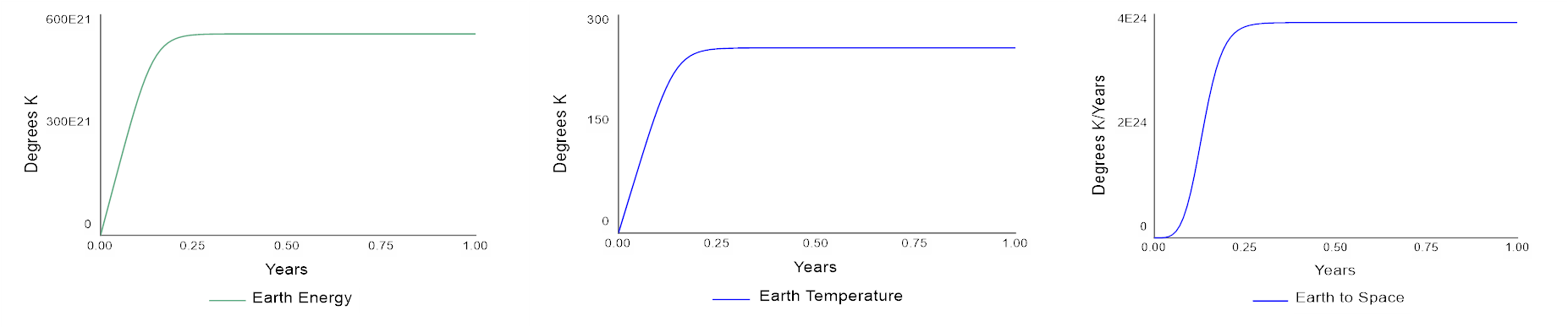
Figure 7
Graphs of Earth’s Temperature (top) and Earth’s energy and Earth to Space radiation (bottom)
Looking at the output graphs, we see that the model in the equilibrium region predicts a radiative equilibrium temperature of 255 K (-18C). This is the temperature that results in a balance between radiation received by the sun and infrared emissions from the Earth.
You will also notice that the curves for Earth Energy (left) and Earth Temperature (center) have the same shape. This happens here because the two variables are in direct proportion to one another (although the actual values are different, as illustrated by the scales shown along the Y-axis). The Earth to Space (2) curve has a different shape because it is proportional to the fourth power of Earth Temperature (T^4). When T is small, relative to its maximum value, the T^4 is very, very small as shown on the lower left corner of the graph; as the two variables approach their maximum values, Earth to Space catches up with Earth Temperature and they both attain their equilibrium values.
|
Units |
|
|
J = Joule |
s = second |
|
m = meter |
yr = year |
|
K = degrees Kelvin |
kg = kilogram |
Table 1
Model units and abbreviations
Part 5: Explore the Model
For your assignment you will be turning in a Word document on Canvas. Include a screenshot of your model structure so far, copy and paste your graphs, and the equations (located under the “MODEL” menu --> "Equation Viewer") into your Word document. Then answer the following questions, also in your Word document.
Question 1
Take a step back and think about the system we are
modeling. To model this system we have made many assumptions. For instance, we
assume that the Earth’s surface is covered by 1 meter of water. As you are
probably aware, this simply isn’t true…but the assumption allows us to simplify
the system. Along this same vein, think about other assumptions we have made in
this model, list three of these assumptions and explain how such an assumption
may affect the model’s output. Were these assumptions reasonable? Note: Take a step back, by assumptions we don't mean specifics of the constants in the model.
Question 2
If you model a different
planet, either closer or further from the sun, than planet Earth,
is the value of the solar constant the same? Why or why not and how does it
change? Finally, do you need to change the structure of the model to
reflect the change in the solar constant?
Part 6: Explore the Solar System
Save the Earth model you created above as “Earth Model”. Next save a second copy of the exact same model, just re-name it the "Venus Model". Now we’ll adjust the ‘Venus model’ to predict the temperature of Venus. We will assume the same Heat Capacity as in the Earth Model, but we will use the Venus Diameter shown in Table 2. **Pay attention to the units (Think: What unit did we originally use for the Earth's diameter?).** Finally, there are two other inputs that need to be modified: Venus Albedo and the Solar Constant (keep reading to figure out how).
Remember that the value for the Solar Constant that we used in the Earth Model was adjusted for the Earth’s distance from the sun. We can re-adjust this for Venus’ distance from the sun by multiplying the function we used by the ratio of each planet’s distance from the sun [Dist2earth/Dist2venus], which is the ratio of Earth’s distance from the sun squared to Venus’ distance from the sun squared (refer to Table 2). The value to be used for Venus Albedo can be obtained from the Internet or another reference source (use the Bond albedo). Be sure to cite your source in your homework.
|
|
Diameter |
Distance |
surface |
surface |
Density |
Main |
|
Sun |
1,392 x 103 |
- |
5,527 |
5,800 |
|
- |
|
Mercury |
4,880 |
58 |
260 |
533 |
5.4 (rocky) |
- |
|
Venus |
12,112 |
108 |
480 |
753 |
5.3 (rocky) |
CO2 |
|
Earth |
12,742 |
150 |
15 |
288 |
5.5 (rocky) |
N2, O2 |
|
Mars |
6,800 |
228 |
-60 |
213 |
3.9 (rocky) |
CO2 |
|
Jupiter |
143,000 |
778 |
-110 |
163 |
1.3 (icy) |
H2, He |
|
Saturn |
121,000 |
1,427 |
-190 |
83 |
0.7 (icy) |
H2, He |
|
Uranus |
52,800 |
2,869 |
-215 |
58 |
1.3 (icy) |
H2, CH4 |
|
Neptune |
49, 000 |
4,498 |
-225 |
48 |
1.7 (icy) |
H2, CH4 |
|
Pluto |
3,100 |
5,900 |
-235 |
38 |
? |
CH4 |
Table 2
Properties of the Planets (note that the units may not match those used in the
model)
**You will need to do a unit conversion!**
Question 3
Again paste a screenshot of your new model structure, the graphs, and the equations for your
Venus Model into your Word document. What value does the model predict for the radiative equilibrium temperature of Venus? (Don't forget to cite your source for Venus' albedo, and include the number you found in your Word document.)
Question 4
Compare the outputs of the Venus and the Earth Model.
Even though Venus is closer to the sun, it has a lower predicted temperature,
why?
Question 5
The radiative equilibrium temperature predicted in our Earth Model differs from the actual surface temperature of today’s Earth (~300 K) by ~40K. Our Venus Model differed from the actual surface temperature of today’s Venus by
>400K. Why does your model miscalculate the actual surface temperatures for Earth and Venus?
*If you're interested in learning more about the topic, feel free to try the Virtual Global Warming Activity.
By the beginning of class next week, please turn in your Word document through the assignments page on your section Canvas site. Your Word document should contain:
- Labeled answers to questions 1 through 5
- Screenshots of Earth and Venus Model structures
- All graphs you have produced
- Equations
Sources
The image at the top of this page is from NASA's Solar
and Heliospheric Observatory
http://photojournal.jpl.nasa.gov/jpegMod/PIA00112_modest.jpg
http://wikyonos.seos.uvic.ca/climate-lab/front_page_pics/temperature.lrg.jpeg