Lab 12- Alteration of the Global Carbon Cycle

Objective

Precise records of past and present atmospheric CO₂ concentrations are critical to studies attempting to model and understand the global carbon cycle and possible CO₂ -induced climate change. Researchers have attempted to determine past levels of atmospheric CO₂ concentrations by a variety of techniques, including direct measurements of trapped air in polar ice cores; and indirect determinations from carbon isotopes in tree rings, analysis of spectroscopic data, and measurements of carbon and oxygen isotopic changes in deep-ocean sediments. The modern period of precise atmospheric CO₂ measurements began during the International Geophysical Year (1958) with Keeling's (Scripps Institution of Oceanography) pioneering determinations at Mauna Loa, Hawaii, and at the South Pole. The Mauna Loa record remains the single most valuable CO₂ time series.

Figure 1

Carbon cycle

In this lab exercise we will do the following:

1. Examine the Mauna Loa CO₂ data.
2. Build a STELLA model of the global carbon cycle in order to understand natural and anthropogenic processes in this cycle.
3. Develop future carbon cycle scenarios and analyze them to determine possible effects on global climate change.

Part 1: Mauna Loa Atmospheric CO₂ Concentrations

Examine the Mauna Loa graph. Notice the seasonal fluctuations. This graph represents the measurement of atmospheric CO₂ concentration (ppm) over time. You will be recreating this in the model below.

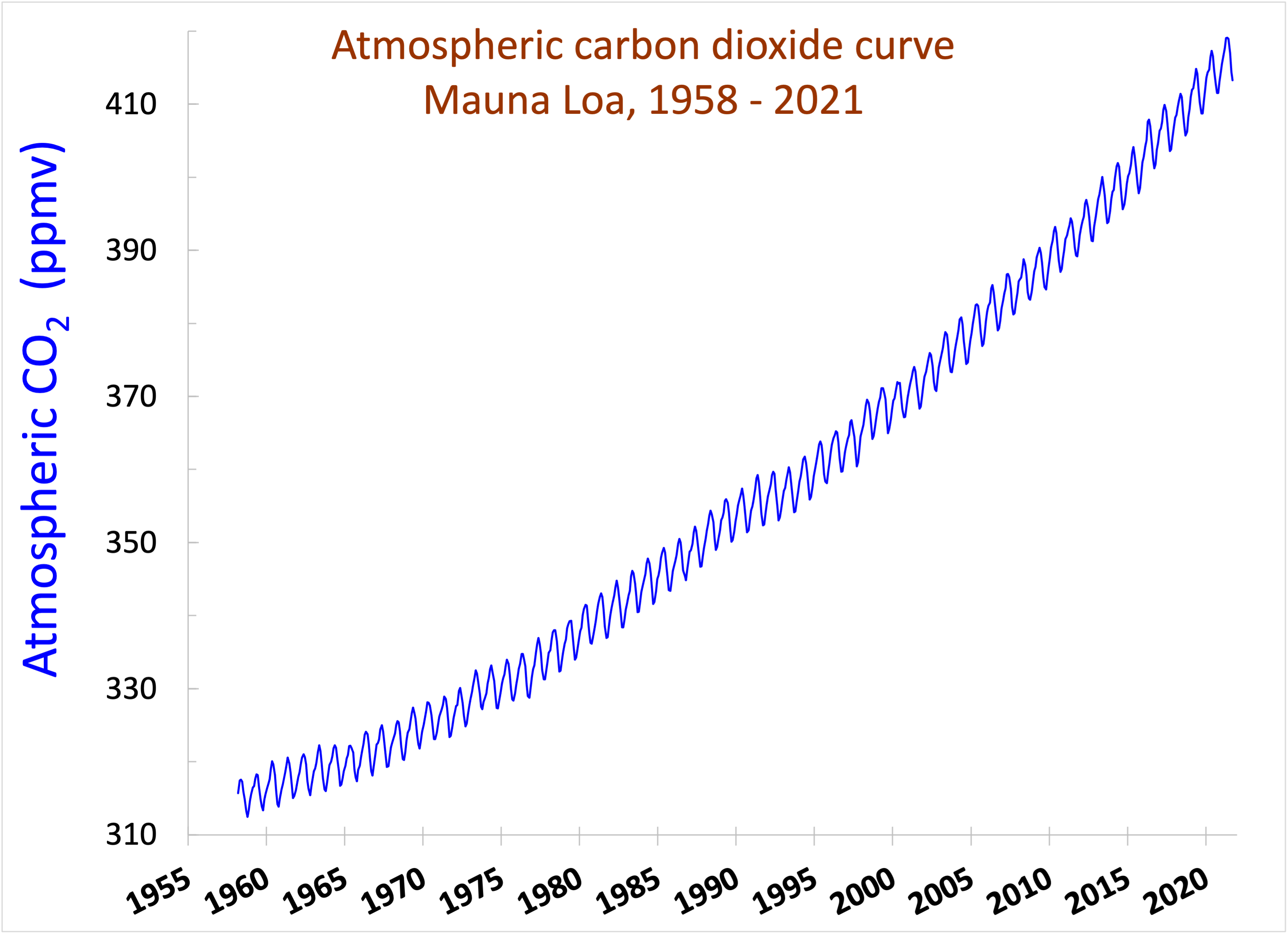
Figure 2

CO₂ concentration from 1958 to 2013

Part 2: Modeling Changes in Atmospheric Carbon Using STELLA

Your next task is to create a working STELLA model of the modern, short-term carbon cycle so that we can understand the patterns and trends in the Mauna Loa curve. Begin by identifying the major carbon reservoirs and the key processes transferring carbon between these reservoirs. Remember that we are exploring the short-term carbon cycle (~50 - 200 years). However, because humans have extracted fossil fuels from sedimentary rocks, we need to include these rocks in our short-term carbon cycle. In groups, draw an outline of your Stella model on paper. You can use the information below as a guide to the reservoirs and processes that need to be included. When you have a complete outline, show it to your GSI and then start building the model in Stella.

Stella modeling reminders!

Make sure you are in model mode.

Begin with placing the stocks.

Next add the flows - to bend flow arrows, hit the Shift key where you want to insert a "kink" in the flow.

[Stella tip: after drawing a flow, you can check the option to make it a "biflow". A biflow allows flow in two directions between two sinks and replaces two separate one-way flows (start your biflow in the Atmosphere). If you use a biflow, you must create converters for each of the one way flows and connect them to the biflow.]

Then add the converters and connectors.

Finally, use the information below to assign initial values to the stocks and flows.

One metric gigaton = 10¹⁵g. (All tons in this lab are metric, also known as tonnes, not U.S. tons.)

Create a numeric display for the Atmospheric CO2 converter.

Note that values provided below may not be the same as those given in lecture. The values below are from 1958, which is the starting point of the model.

Stock #1: Atmospheric Carbon

Initial Value (1958) = 720 {gigatons}

Inflows

• Ocean Release = 105 {gigatons/yr.}
• Plant Respiration = 60 {gigatons/yr.}
• Deforestation = 1.8 {gigatons/yr.}
• Soil Respiration = 60 {gigatons/yr.}
• Fossil Fuel Combustion = 5 {gigatons/yr.}

Outflows

• Ocean Uptake = 106.6 {gigatons/yr.}
• Photosynthesis = 80 + NH Photosynthesis {gigatons/yr.}
• Unknown Sink = 2.2 {gigatons/yr.}

Stock #2: Land Plants

Initial Value (1958) = 560 {gigatons}

Inflows

• Photosynthesis (see above)

Outflows

• Detritus = 60.4 {gigatons/yr.}
• Deforestation (see above)
• Plant Respiration (see above)

Stock #3: Ocean Carbon

Initial Value (1958) = 38000 {gigatons}

Inflows

• River Transport= 0.8 {gigatons/yr.}
• Ocean Uptake (see above)

Outflows

• Sediments = 0.1 {gigatons/yr.}
• Ocean Release (see above)

Stock #4: Soils

Initial Value (1958) = 1500 {gigatons}

Inflows

• Detritus (see above)

Outflows

• Soil Respiration (see above)
• River Transport (see above)

Stock #5: Sedimentary rocks

Initial Value (1958) = 75000000 {gigatons}

Inflows

• Sedimentation (see above)

Outflows

• Fossil Fuel Combustion (see above)

Converters

• Atmospheric CO2 ppm = 310 * (Atmospheric Carbon / 720)
• NH (Northern Hemisphere) Photosynthesis = PI*40*MAX(0,SIN(2*PI*(Season-0.25))) (Use the built-ins to input this)
• Season = TIME-INT(TIME) (Use the built-ins to input this)

Run Specs

Change the Run Specs so that the simulation runs from 1958 to 2013 (corresponding approximately with the Mauna Loa data), using a time step (DT) of 0.05 years.

Questions

Question 1 (2 points)

Run the model and graph Atmospheric CO2 concentration (in Stella). Paste your first graph from 1958-2013 into your WORD document. Explain the annual seasonal variation that you built into your model and that you see in the Mauna Loa graph. What is the biological mechanism for this cyclical fluctuation? Although the graph our model produces does not show this, in reality (see the Mauna Loa graph above) the seasonal difference between maximum and minimum CO2 concentrations has been increasing over time. What could cause this increase?

Question 2 (3 points)

2a. Look on the internet and find the current input of fossil fuel carbon to the atmosphere. You can download a data file at this site. Make sure that your units are compatible. Use this in your stella model and include a graph of the result. How does this compare to the real Mauna Loa curve (in both magnitude of increase and trend)?

2b. If your model does not exactly match the Mauna Loa graph how might you make it more realistic (Hint: fossil fuel inputs were not the same in 1958 as they are today. You might try using a graphical function to make the fossil fuel inputs more realistic.) Update your model to make it more realistic. Explain what you did and include a graph.

Question 3 (3 points)

Look at the processes in the global carbon cycle and identify the anthropogenic (human-made) factors. By altering one or more of these, develop a possible future scenario of the carbon cycle and model it in STELLA (you can make this realistic by looking up values on the web). First change your run specs to go into the future (from 1958 to 2100) then alter your chosen anthropogenic features. Include your new (relabeled) graph of Atmospheric CO₂ (ppm). Describe the factors you changed and how these changes affected the atmospheric global carbon curve with time. Note how long it takes in your different scenarios to double the atmospheric CO₂ concentrations. How realistic are your scenarios and the changes you made given our current global society?

Question 4 (2 points)

Given the mass balance calculations that have been done with known concentrations of atmospheric carbon, we need a "sink" to balance the global C budget. In other words, we are "missing" over 2 billion tons of C each year; this shows how incomplete our understanding of the global carbon cycle is at present. What are some of the scientific speculations about where this missing sink could be located? Name at least two.

Make sure to include all of your graphs (should be 4 of them), your final model, and the final equations with the answers to the questions in your homework assignment. Make sure to submit it as one WORD document as an attachment on Ctools. Please make sure to label all your graphs!

Sources

Pew Center for Climate Change Report: Land Use & Global Climate Change (June 2000). Chapters II and III will be most useful (p. 5-25).

http://www.c2es.org/science-impacts/ipcc-summaries/fourth-assessment-report-summary

Classroom of the Future, Earth on Fire Modules: Carbon Cycle.

http://www.cotf.edu/ete/modules/carbon/efcarbon.html

http://www.ucar.edu/learn/images/carboncy.gif

Back to index