Long-term Climate Regulation
OBJECTIVES
The objectives for this lab include improving your skills at modeling, which you will need for your final class project, and developing an understanding of how the Earth’s carbon cycle has changed over time, and how it has affected climate by changing our planetary energy balance. This theme was introduced early in the lectures for the class, and at this point in the semester we are ready to synthesize the two main themes of carbon cycling and Earth's energy balance by combining elements of the carbon cycle lab and the energy balance lab. In terms of the potential applications of such a task, consider that you are employed as a systems analyst at an international company working on providing sustainable, integrated plans for environmental protection and restoration in a large country in, e.g., Africa or S. America or Asia (etc.). Your boss has asked you to explain how the “system” of global temperature, greenhouse gases, and planet energy balance actually operates, and not just in the present but over very long periods of time. You are borrowing from Earth’s history in order to produce a sustainable plan, and your task is to look at millions of years of history and describe how the “system” operates, which is the gateway task needed to develop the environmental protection and restoration plan your company needs.
1 Introduction
Earth’s climate has changed through time. There have been ice ages and ice-free periods. Yet, for most of Earth’s 4.5 billion years, the temperature has been hospitable, not too cold nor too hot for life of some kind. The regulation of climate through geologic time has been attributed to interactions between the climate system and the carbon cycle. In this lab, you’ll investigate these interactions and how they have regulated Earth’s climate.
Long-term
carbon cycle
The carbon cycle describes
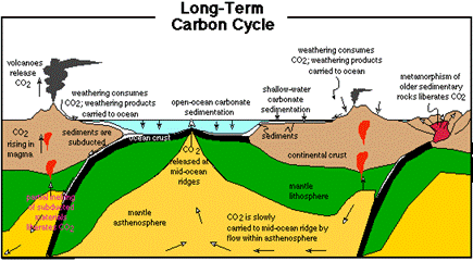
changes in the fluxes and reservoirs of carbon in the Earth system (Fig. 1). On
very long time-scales, millions of years, the primary reservoirs of carbon are
the atmosphere, ocean, and rocks (limestone). Carbon moves between these
reservoirs through volcanic outgassing, silicate weathering, and limestone
sedimentation. The carbon cycle is linked to Earth’s energy balance through atmospheric
carbon in the form of CO2, a greenhouse gas.

Fig. 1.
Schematic of the long-term carbon cycle (from Bice, 2001)
Earth’s
energy balance
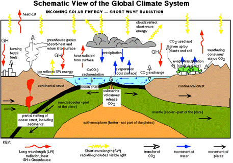
As you learned in the Energy Balance Lab, the
energy balance between incoming shortwave radiation and longwave outgoing
radiation determines Earth’s climate (Fig. 2). The net incoming shortwave
radiation is influenced by the Sun’s luminosity and Earth’s albedo. The net
outgoing longwave radiation is a function of Earth’s temperature (through
black-body radiation) and the greenhouse effect. Earth’s climate affects the
carbon cycle through temperature, which modifies the rate of silicate
weathering and the rate that carbon dioxide is removed from the atmosphere.

Fig. 2. Schematic of the climate system (from Bice, 2001)
2 Exploring the Long-Term Carbon Cycle
A model of the long-term
carbon cycle has already been developed for you. This model was designed
by David Bice (2001). Start by opening the Stella model (carboncycle model you must right click and save link as). In its current form, the carbon
cycle is not linked to the climate system. This is a good place to start in
order to understand how the long-term carbon cycle works without the
complicating influence of climate.
Model Operation Notes:
Note the following abbreviations for this model: ATMOS = atmosphere, C
= carbon, DT = delta temperature, SW = short wave, LW = long wave, SURF = surface, SFC = surface, Gt =
gigaton, ABS = absorption.
Table 1. Carbon model run spec
parameters. (Note: DT here is the time step)
Length of Simulation DT (Myrs)
Integration
Method 0 to 10 (Myrs)
0.005 RK2 (Runge-Kutta 2)
Q
1. The
response time is how long the system takes to
re-establish steady state after a perturbation. Double the ATMOS C reservoir from 600 Gt C (gigatons of carbon) to 1200 Gt C.
Run the model, again graphing ATMOS C,
OCEAN C, LIMESTONE. What is the response time of the long-term carbon cycle?
Remember that time here is in millions of years. Where did the excess carbon
end up? Did it remain in the ATMOS C
reservoir? Explain this result using concepts from class.
(2.5 points) Q
2. Return the ATMOS C reservoir
to its initial condition so that you can test how the model responds to a
temperature perturbation. First, make your own prediction. Next, test your
prediction. Increase the external DT
converter to 1. This represents a 1 K (1 °C) increase in global temperature.
Run the model. Graph ATMOS C, OCEAN C, LIMESTONE. How did the distribution of carbon between reservoirs
change after increasing the external DT? Why? Explain your answer in terms of changes in carbon fluxes between
reservoirs. You must support your answer with numerical results from the model.
(2.5 points) A model of the Earth’s
energy balance has already been developed for you as well. This model was also
designed by David Bice (2001) at
Check to confirm that your Run
Specs are the same as those in Table 2 below. Graph SFC TEMP (Surface Temperature). Run the model. The
model should be in steady state.
Table 2. Climate model run spec
parameters Length of Simulation DT Integration
Method 0 to 10 (yrs)
0.01 RK2 Q 3. Our primary goal in this lab
is to investigate climate-carbon cycle interactions. To begin, explore how the
climate system responds to perturbations in the absence of the carbon cycle.
Let’s perturb the system by changing the Solar
Input, the percent of Sun’s radiation received by Earth. This experiment
isn’t entirely unrealistic. Remember that Sun’s luminosity has increased with
time at a rate of 1% per 100 million years. Run the model (a new run each time) trying values of 99, 98, 97, 95, 80. Set your numeric value tool to display SFC DT, and set the precision to 0.00 (two decimal points). Record this value in the
table below. Summarize in words what the
table means.
Solar Input SFC DT 100 0.00° 99 98 97 95 80 ***Return
Solar Input from your model to 100 before the next step.*** 4. Climate Regulation by
Carbon Cycling
Now,
it’s time to link our carbon cycle model and our energy balance model. This requires
a fair amount of manipulation in Stella, excellent practice for you to hone
your modeling skills. Start
by copying and pasting the entire energy balance model into the window with
your carbon cycle model using the tools in the Edit menu. Note: Put the Energy Balance model that we give you in this lab into the Carbon Cycle model (not the reverse). Hint: Use Edit -> Select All, then Edit -> Copy. Hint: before pasting, click in the far corner of your model space so that your models don't overlap.
To link the models, you need
to make a few modifications: (1) Delete the SFC DT and external DT converters from the
carbon cycle model.
(2) Create a radiative forcing converter and connect
it to the LW SPACE flow. Also connect
the relative atmos C converter to the
radiative forcing converter. Double
click on the new radiative forcing
converter and add the following equation: 5.35*LN((relative_atmos_C + 0.0000000000001)/280)
This equation defines the
relationship between CO2 and radiative forcing. The relationship is
logarithmic. As atmospheric CO2 increases, the radiative forcing
increases by a smaller and smaller amount. (3) Double click on the relative_atmos C converter. Modify the
equation by multiplying by 280 (the pre-industrial concentration of CO2).
It should read: (ATMOS_C/600)*280 (4) Modify the LW SPACE equation to include the radiative forcing from the carbon cycle
model, and multiply this term by 10 (see explanation in step 6). The equation
should be: (60*((ATMOS_TEMP/255)^4) –
radiative_forcing)*10 (5) Rename SFC DT_1 to SFC DT. Connect the SFC DT
converter to weathering.
(6) And, finally, multiply
the SW ATMOS, SW SURF, LW ATMOS, LW SURF, and the SFC LW SPACE flows by 10 (put the existing equation in parentheses
" ( ) " first!). This is a little sleight of hand. The energy balance model and the
carbon cycle model operate on very different time scales (years versus millions
of years). As far as the carbon cycle is concerned, the atmosphere responds
immediately. However, Stella requires that the models operate on the same, long
time scale. By multiplying the energy balance fluxes by 10, we’re essentially
running the climate system on a slightly shorter time scale. This trick isn’t
perfect, but will work as long as our focus is the steady state answers.
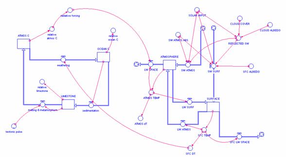
Fig. 3.
Schematic of the climate-geochemical model in Stella. Check to confirm that your
Run Specs are the same as those in Table 3. Also make sure that you returned
the Solar Input to 100. Run the
climate-geochemical model. Graph SFC TEMP.
The model should have a steady state temperature of 288 K. Table 3. Model run spec parameters Length of Simulation DT (Myrs)
Integration
Method 0 to 20 (Myrs)
0.005 RK2 Q 4. Let’s compare solutions from
our climate model (energy balance model) with our climate-geochemical model. As above, perturb the
system by changing the Solar Input.
Again use values of 99, 98, 97, 95, 80. Record the change in Earth’s surface
temperature (SFC DT) in a table.
Compare the solutions using the climate model (energy balance model) and the coupled climate-geochemical model. Explain why the solutions are
different. Specifically address how climate-carbon cycle interactions affect
the final global average temperature. (Hint: Remember that this lab focuses on the long-term carbon cycle). (2.5 points)
Solar Input SFC DT 100 0.00° 99 98 97 95 80 Lab Assignment: Turn in a Word document on Canvas that includes answers to all 4 questions and include the 2 tables. Make sure to number and label your tables.
1. Check to confirm or change your Run Specs so they are the same as those in Table 1 below. In addition, change “Sim Duration” to at least 5 seconds so you can see how carbon flows through all three stocks in the numerical displays
2. Make Graph 1, which includes the variables ATMOS C, OCEAN C, LIMESTONE. In graph settings, check "Multiscale". Create numeric displays (figure 8 button) with 'full precision' in the formatting option for each of these variables as well. Run the model. The
model should be in steady state. Note the different sizes of the carbon reservoirs.
3. Settings: For each numerical display (ATMOS C, OCEAN C, LIMESTONE), insert the display, select one of the variables, and click “Formatting” from the dropdown arrow. Then, under the “Precision” option, change “Auto precision” to “Full precision”. This is the only way you’ll be able to see the changes in the Ocean and Limestone carbon stocks.
3 Exploring the Climate System
