Gaia and Daisyworld
Introduction
In class so far we have learned how Earth's radiative energy balance is controlled by incoming energy from the sun, reflected energy (albedo), and outgoing energy released from Earth back to space. In addition, we know that the Earth's energy balance is modified by the "greenhouse effect", where heat-trapping gases such as carbon dioxide in the atmosphere may increase and warm Earth, or decrease and cool Earth. Changes in Earth's climate over the geological timescale of 100s of millions of years have been regulated by volcanic activity increasing carbon dioxide, and silicate rock weathering decreasing carbon dioxide in the atmosphere. But there are still changes in Earth's climate that cannot be fully explained by volcanoes and weathering, and that may be related to the evolution and activity of life on our planet. In this lab we will investigate the potential role that life might have on Earth's climate.
In the 1960s, James Lovelock was employed by NASA to help determine whether life existed on Mars. While Lovelock’s colleagues were inventing methods of detecting life on Mars, Lovelock argued based on the known composition of Mars’ atmosphere that it couldn’t contain life.
Lovelock noted that the atmospheric compositions of Venus and Mars are similar and are close to chemical equilibrium. In other words, there is no imbalance, or no net production or destruction of chemical components. In contrast, Earth’s atmospheric composition is not at chemical equilibrium. (Note in Table 1 below how different Earth’s chemical composition is from that of Venus and Mars.) The persistence of an atmosphere in chemical disequilibirum, and at a relatively constant composition for time periods longer than the reaction times of the gases, implies that the Earth’s atmosphere is somehow “regulated” - and the regulating mechanism is life.
Table 1. Chemical composition of terrestrial planets.
| Atmos. Composition |
Venus |
Earth |
Mars |
CO2 |
96% |
0.04% |
95% |
N2 |
3.4% |
78% |
2.7% |
O2 |
0.0069% |
21% |
0.013% |
H2O |
0.3% |
0-4% |
0.03% |
From this early observation of some regulation of Earth’s atmosphere, Lovelock and his colleagues formulated the Gaia hypothesis. What is Gaia? Gaia is a self-regulating system composed of the Earth’s climate and environment that is a consequence of an automatic, but not necessarily purposeful, goal-seeking system. Gaia has also been described as a super organism, analogous to a beehive that has the goal of maintaining an environment suitable for its own existence.
According to Lovelock, Gaia is composed of at least four elements:
- Living organisms that exploit any environmental opportunity,
- Organisms that follow Darwinian natural selection,
- Organisms that affect their physical and chemical environment, and
- The existence of constraints to the limits of life.
The Gaia hypothesis has rather astounding implications. It suggests that:
- Life is a planetary-scale phenomenon.
- There can be no partial occupation of a planet by living organisms; total occupation is needed for adequate regulation.
- The evolution of organisms and the evolution of the environment are intimately and irreparably linked.
- Increased biological diversity could lead to better regulation (more stable, or more sustainable- this will be addressed in later lectures).
After first proposing the Gaia hypothesis, Lovelock encountered many critics. The main criticism was that Gaia is teleological. That is, it requires organisms to have a collective purpose. In addition, it was known that biological regulation is only half the story. The evolution of the atmosphere involved the co-evolution of organic (biologic) and inorganic components.
Formulation of the Daisyworld model
In response to his critics, Lovelock invented the Daisyworld model to demonstrate that self-regulation could occur without a collective purpose. Daisyworld is a simple Earth-like world that is inhabited only by white daisies. (Yes, that’s right, the flower.) The temperature of Daisyworld is determined by the fraction of the planet covered by daisies and the fraction that is bare soil. Because of their white color, daisies have a high albedo (reflectivity). The dark, bare soil has a lower albedo. The planetary temperature of Daisyworld can be calculated if the fraction of daisies is known. In the rest of this section, we describe the details of the Daisyworld model. There is some algebra involved, but it looks more daunting than it actually is. You saw these concepts last week in class.
Figure 1. The white daisy, inhabitant of Daisyworld, in all of its glory.

To calculate the planetary temperature, radiative equilibrium is assumed (this equilibrium is achieved much more rapidly than the sun changes its luminosity). Radiative equilibrium assumes that the energy emitted by planetary longwave radiation is equal to the shortwave radiation received from the Sun. In the absence of radiative equilibrium, the planet will warm or cool until radiative equilibrium is established.
Energy emitted = Energy absorbed (equation 1)
The energy emitted is simply defined by the Stefan-Boltzmann Law, which states that the energy emitted from a body is proportional to the fourth power of the body’s temperature:
Energy Emitted = A * ε * σ * T4 (2)
In equation (2), A, ε, σ, and T are Daisyworld’s area, emissivity, the Stefan-Boltzmann constant, and temperature, respectively. The energy received by Earth (aka energy absorbed) is the energy received that is radiated from the Sun minus the portion that is reflected back to space:
Energy Absorbed = Energy Received – Energy Reflected (3)
The energy reflected is a function of how many daisies there are. More white daisies increase the planetary albedo (i.e., reflectance), thereby causing more sunlight to be reflected back to space and preventing the sunlight from warming the Earth.
Energy Reflected = Planetary Albedo * Energy Received (4)
The planetary albedo is calculated by multiplying the total fraction of Earth that is either daisies or soil by the albedo for each surface:
Planetary Albedo = fdaisy * αdaisy + fsoil * αsoil (5)
In equation 5, f is the fraction of Daisyworld that is either soil or daisies, and α is the albedo of these surfaces. If Daisyworld is completely covered with flowers, the fraction of daisies (fdaisy) will be 1 and the fraction of soil (fsoil) will be 0.
The above equations describe the relationship between the planet’s temperature and the fraction of daisies. In addition, an equation is needed to express the conditions for the growth of daisies. On Daisyworld, it is assumed that the planetary temperature determines whether and how fast daisies grow. Daisies can survive at temperatures between 5 and 40 ºC, but do best at temperatures near 22.5 ºC. This relationship is expressed through a complicated-looking growth factor:
GFdaisy = 1- 0.003265 *(22.5 – Tdaisy)2 (6)
When equation 6 is plotted it should look like this:

The temperature of the daisy-covered areas, Tdaisy, is written as:
Tdaisy = FHA * ( αplanet – αdaisy) + Tplanet
(7)
This equation, where FHA is a heat absorption factor, converts sunlight (energy) into temperature. Finally, it is necessary to convert the growth factor into an expression of the change in the area of daisies. The change will be represented as:
Area change = Areadaisy * ( Areasoil * growth factor – death rate) (8)
This expression consists of two elements. First, it gives the area lost through a constant death rate (-Areadaisy * death rate). Second, it expresses the area gained through daisy growth (+Areadaisy * Areasoil * growth factor). This last term is written such that the optimal growth will occur when there is an equal area of daisies and soils. Growth will slow both with less daisy area (fewer flowers to germinate) and with more daisy area (no bare ground in which to grow).
Concept of Equilibrium States
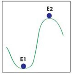
Many systems, including the climate system, are thought to have equilibrium states. An equilibrium state is a state of no change. The classic example of equilibrium states is that of a ball on an uneven terrain (Fig. 2). In this example, the equilibrium states exist when the ball is either in a valley (E1) or on a hill (E2). There are two types of equilibrium states, stable and unstable. In an unstable equilibrium (E2), a small perturbation to the system (a small push on the ball) will cause the system to move to a new equilibrium (the valley in Fig. 2 - note that this is NOT reversible; that is, if you give another small push on the ball it will not return to it's original state of being on the top of the hill where it started in the E2 position). In a stable equilibrium (E1), a small perturbation to the system will not alter the equilibrium state. Rather, the ball will return to its original position (E1). One of the most important questions facing us is whether our climate system is stable or unstable. If the climate system is unstable, a perturbation to the system (such as warming caused by carbon emissions) will send it into a very different state.
Figure 2. Classic example of equilibrium states. E1 represents stable equilibrium; E2 represents unstable equilibrium.

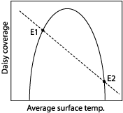
Daisyworld also has equilibrium states. They can be determined by comparing the effect of temperature on the daisy coverage (solid line) and the effect of daisy coverage on temperature (dotted line). The intersection of these curves at E1 and E2 represents the equilibrium states.
Figure 3. Relationship between daisy fraction and temperature. The lines intersect at equilibrium points (E1 and E2).

To determine whether the equilibrium states are stable or unstable consider the response of the system at E1 to a small negative temperature perturbation. Such a small perturbation will cause the daisy coverage to decline and the planetary albedo to decrease slightly. With a small reduction in albedo, the surface temperature will warm. As a result, the system eventually returns to its E1 state. Similarly, a small positive temperature perturbation will cause the daisy coverage to increase, increasing the planetary albedo, and reducing the temperature. E1 is a stable equilibrium.
Now consider a negative temperature perturbation at E2. In this case, the daisy coverage increases, the albedo increases, and the temperature is reduced even more! The system is moving away from the equilibrium position at E2. This equilibrium is unstable.
Assignment: Wreaking Havoc on Daisyworld
Now that we understand the basics of Daisyworld, let’s mess with our model! Our goal here is to evaluate the Gaia hypothesis, and particularly to determine whether biological regulation of climate is possible or whether it requires divine intervention as the critics of Gaia have argued.
For the sake of time, we have already constructed the Daisyworld model for you, right-click on this link and save it to your Google Drive or U-M Dropbox: WhiteDaisyWorld.stmx
- Begin by opening the file named WhiteDaisyWorld.STMX. This is a dynamic model (change in time) and it is important to understand that the model has an equilibrium state.
- Create a graph to show the White Daisy Fraction and Soil Fraction. Now run the model.
- Give your graph the title "Graph 1: Soil vs. Daisy Fraction" and rename the X Axis as "Millions of Years" (graph settings)
- Click on the graph and drag left and right to see the values for the variables over time.
Question 1. Answer all the following questions and include "Graph 1: Soil vs. Daisy Fraction" from above: Is the system in equilibrium? How do you know? What is the equilibrium white daisy fraction? The soil fraction?
Now we’ll adjust our model for the evolution of Earth's climate. Our Sun has become more luminous since it formed.
- To simulate the Sun’s evolution, click on the Solar Luminosity converter. Place {} around 1.0 (Stella ignores anything within brackets, {}, so this will keep stella from using the 1.0 value.)
- Delete the {} surrounding the equation for solar luminosity. (Stella will now recognize this as the new formula to use.)
- Make a new graph of the solar luminosity, planetary temperature, dead planet temperature (the temperature the planet would have in the absence of daisies), and the White Daisy fraction. Adjust your graph settings to observe the dynamics of the shift by selecting "Multiscale". Title as "Graph 2: Solar Luminosity"
- Run the model and copy the graph to your Word document for Question 2. Click on the graph and drag left and right to see the values for variables over time.
Question 2. Answer these three subquestions: What is the effect of an increase in solar luminosity over time on the white daisy population? What is the mechanism that allows daisies to affect the planetary temperature? Explain, using equilibrium concepts, how and why the daisy population changes. [Hint: think about stable and unstable equilibrium points discussed earlier] Include “Graph 2: Solar Luminosity”.
Keep the solar luminosity function the same as from Question 2. The Optimal Growth Temperature (set at 22.5°C) is the preferred temperature for daisy growth. This factor is determined empirically, or assumed.
- Try altering the optimal growth temperature, and plot white daisy fraction.
Question 3. Answer these questions and include your completed table and one representative graph: How does the optimal growth temperature affect the timing of equilibrium? Why? Copy the table below to your Word document, record your results for different alterations of the Optimal Growth Temperature then use the table to help you answer the question.
Optimal Growth Temperature |
Time of White Daisy Growth (myrs) |
Time of White Daisy Death (myrs) |
|
|
|
|
|
|
|
|
|
In the "Time of White Daisy Growth" column, include the year when the daisy population began growing. In the "Time of White Daisy Death" column, include the year when they daisy population dropped to zero.
Now let’s add a little ‘man-made’ cataclysmic variability to the system by including a plague in the Daisyworld model. Make sure the optimal growth temperature is 22.5°. This work will allow you to answer Question 4.
- Click on the Death Rate converter. To simulate a plague, we want to make the death rate a function of time.
- To do this, replace 0.3 with TIME in the equation box from the built-in options.
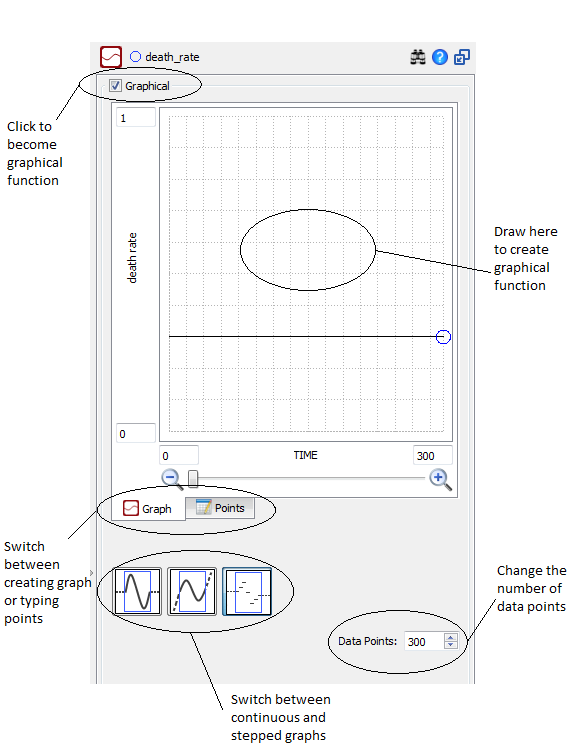
- Now switch from equation mode to graphical function mode by first clicking on the graphical function tab.
 These tabs are located on the bottom right-hand side of the screen in the same panel as the equation box (not in the upper toolbar). Then, click the 'Graphical' checkbox at the top of the Graphical function panel that opens.
- First we'll reestablish the base death rate of 0.3 before introducing our changes.
- Choose the 'Points' tab in the Graphical Function panel.
- Change the number of 'Data Points' to 2.
- Click each value in the death rate column and type 0.3.
- Now change the 'Data Points' to 30, all will have the same 0.3 value now.

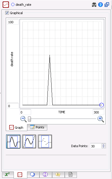
- Now we’ll add a plague. Ensure you're in the continuous graph mode by clicking on the leftmost graph function. The first plague we will add will peak at year 103.448 (in the ‘TIME’ column in the "Points" tab).
- To add a plague, go to the Points tab and change the death rate at this time to 60.
- Notice this plague only lasts for ~20 myrs (from 93 to 113 in the graph). If you click on the Graph tab it should look like this:

Run the model and graph the White Daisy Fraction and the planetary temperature. Title the graph as "Graph 3: Plague". Think about how the daisies respond to this plague, and think about how the plague affects the planetary temperature.
Now we’ll explore the effects of plague timing and plague magnitude. In the table below we have provided three scenarios for you to observe. In the steps above you have already completed the first scenario. To complete the subsequent scenarios, reset all death rates to 0.3, prior to adding a new plague.
- Note that the final three scenarios are of your own choosing. Be creative. Perhaps allow the plagues to last for more than 20 myrs, or perhaps unleash 2 plagues during one model run. It is up to you.
- For each scenario in the table, run the model and fill in the table below with your results.
- Feel free to graph more variables if you think it will help you understand the system better.
Question 4: Answer the following questions: Does each plague respond similarly in magnitude and planetary temperature change? Why or why not? Explain your observations in terms of equilibrium concepts. Include your table from below with all values filled in. Also include ONE representative "Graph 3: Plague" in your Word document.
| Plague Death Rate |
Year of Plague (myrs) |
Duration of Plague (myrs) |
White Daisy Response |
Temperature Response |
60 |
103 |
20 |
|
|
90 |
103 |
20 |
|
|
60 |
155 |
20 |
|
|
| |
|
|
|
|
| |
|
|
|
|
| |
|
|
|
|
In the "White Daisy Response" column, include the years when the daisy population size decreased or went to zero. In the "Temperature Response" column, describe how the temperature changed and at what years.
Question 5. Let’s think about what we have learned from the Daisyworld model. We’ve seen (in Question 2) that the daisies can control the planetary temperature. Answer the following questions - these are not "Yes or No" questions, they require thought and reflection (no more than 1 paragraph typed for each of the 3 questions parts below):
- Was there any design or collective purpose on the part of the White Daisies to take over the planet and modify the temperature, or said another way, did the daisies have knowledge of their influence?
- Part of this lab involves thinking critically about the Gaia hypothesis and what evidence exists to support or refute its claims. In considering this more broadly, what counts as evidence for or against a (any) hypothesis? How do your own societal, cultural, and lived experiences shape what you consider to be "evidence" for or against any hypothesis?
- How do models help you simplify aspects of physical, biological, chemical, social, or other complex systems? (Remember that models are not always mathematical, they could be conceptual such as diagrams or pictures.) Conversely, what are some limitations in models, and what can we learn despite the limitations?
Lab 3 Assignment
By the beginning of next week's lab, on your section's Canvas site, please turn in the following in a single Word document.
- Answers to questions 1 through 5.
- Copies of the graphs for Questions 1 and 2.
- Completed tables for Questions 3 and 4.
- Choose a representative graph from EACH of Q3 and Q4 to include with your answer.
References
Bice, D., 2001, Exploring the Dynamics of Earth Systems: Models Using Stella, http://specialpapers.gsapubs.org/content/413/171.full
Lovelock, J., 1988, The Ages of Gaia, W.W. Norton & Company, New York, 255 pp.


